The properties of an electron can be described by a mathematical function called wave function (ψ). There is a radial and an angular part of every wave function. As the radial wave function changes sign from positive to negative, it crosses the x-axis and that point where ψ=0 is called a radial node. Angular nodes can be found by looking at the 3D diagram of the atomic orbitals. An angular node exists in a plane where the electron density is zero. For example,

This is an s orbital. It has no angular node as all the planes intersect the orbital.

These are p orbitals. They each have one angular node, which occurs on the plane which doesn’t touch the orbitals i.e. xy plane for 2pz, yz plane for 2px and xz plane for 2py.

These are d orbitals. They each have two angular nodes, again occurring on the plane that doesn’t touch the orbitals, i.e. yz and xy planes for 3dxz, xy and xz planes for 3dyz, xz and yz planes for 3dxy, planes bisecting the xz and yz planes for 3dx2-y2 and for 3dz2 are the two cones in the z axis facing in opposite direction with their vertices meeting at the origin, as shown in picture on the right

The total number of nodes (angular + radial) is equal to n-1, where n is the principal quantum number. Hence,
1s orbital has no angular no radial node
2s orbital has no angular node and one radial node
2p orbitals have one angular node and no radial node
3s orbital has no angular node and two radial nodes
3p orbitals have one angular node and one radial node
3d orbitals have two angular nodes and no radial node
and so on.

Therefore, by knowing the 3D shapes of the orbitals and therefore the number of angular nodes, we can find out the number of radial nodes the orbital has, which corresponds to the graphs below.

Molecular orbitals resulting from combining atomic orbitals can be constructed in phase (ψ+) and out-of-phase (ψ-). In phase addition occurs when the wavefunctions of the two atomic orbitals combined are of the same sign. For example, in the simplest case of 1s AO which is positive, adding two such AO will lead in a constructive interference. A bonding MO is thus formed. Similarly subtracting the AOs leads to a destructive interference forming an antibonding MO.

In the region between the two nuclei in in phase addition the value of the MO wavefunctions is greater than that of the AO wavefunctions. Thus it is more like likely to find an electron in the inter-nuclear region.   
The in-phase MO is lower in energy than the isolated AOs because:
1. When the MO is occupied, there is increased electron density between the nuclei. The attraction from both nuclei leads to a lowering of the potential energy of the system.
2.  An electron in in-phase MO is less constrained compared when in an AO (i.e. it is more delocalized) leading to a decrease in its kinetic energy.
The in-phase combination MO is lower in energy than the original AO and occupancy of this orbital gives rise to bonding, thus this orbital is called the bonding molecular orbital.

For the out of phase addition, the anti-bonding combination has a node – where the electron density is zero. This is shown by the crossing point on the x axis (horizontal line).
    
The out-of-phase MO is higher in energy than the isolated AOs because:
1. When the MO is occupied, there is much more electron density outside the inter-nuclear region than in between the nuclei pulling them apart from each other. The potential energy in this MO is therefore higher than in the separate species.
2. The out-of-phase MO contains a node. This means that the kinetic energy of the electron in this orbital is greater than when it is in either the AO or in-phase MO.
The out-of-phase combination MO leads to an increase of the energy with respect of the original AO, thus this orbital is known as the anti-bonding molecular orbital.

This can be summarized graphically using an energy level diagram:

The Molecular Orbital Theory (MO Theory) is necessary as it presents some distinct advantages over the valence bond theory (VB Theory). Figure 4.1 below will detail the differences between MO theory and VB theory:

Figure 1.1: Table comparing VB theory to MO theory

As seen, the MO theory is much more effective in explaining formation of bonds between atoms than the VB theory.

It has been mentioned previously that the number of molecular orbitals formed is the same as the number of atomic orbitals involved in bonding. The total number of electrons in the molecular orbitals is therefore also the same as the number of electrons in the original atomic orbitals.

The filling of electrons into the molecular orbitals follow three basic rules:

1. The Aufbau principle: Electrons are filled from the lowest energy orbital to the highest energy orbital. For example, atomic orbitals in atoms are filled from lowest energy to highest energy according to this order: 1s < 2s < 2p < 3s < 3p < 4s < 3d < 4p < 5s < 4d < 5p < 6s < 4f < 5d < 6p < 7s < 5f
2. The Pauli Exclusion principle:
   • No more than two electrons can occupy one orbital
   • The two electrons must be of different spins
3. Hund’s Rule: When there are degenerate orbitals, electrons will occupy empty orbitals before pairing up with another electron to minimize repulsion between particles of like charges

The following very interesting video will explain these three basic rules:

Now that we have seen the usefulness of MO theory over valence bond theory, let’s take a look at how we can use the theory by finding the bond order of a molecule.

Previously, we have learnt how to fill the molecular orbitals following the Aufbau’s principle, Hund’s Rule and the Pauli’s Exclusion Principle. Now, we are going to use that molecular orbitals diagram to find the bond order. Read on to find out how!

Bond order

The concept of bond order in layman terms can be described as the average number of electrons involved per bond in a molecule.

It is based on the formula, B.O. = ½ [ no. of bonding electrons – no. of anti-bonding electrons].

As an example, let’s look at oxygen below.

MO Diagram of Oxygen

Bond order in O2 = ½ [ no. of bonding electrons – no. of anti-bonding electrons] = ½ [ 10 – 4 ] = 2

Hence an average of 2 electrons are involved in a bond in O2.

In reality, the dot and cross diagram does prove that to be true, as shown below.

You may want to try calculating the bond order for other molecules.

Try the example below:

Fluorine MO Diagram

Remember, bond order in O2 = ½ [ no. of bonding electrons – no. of anti-bonding electrons]

Answer: B.O.= 1

The bond order generally tells us the strength of the bond. The higher the bond order, the stronger the bond. We may make use of bond strength to further discuss about the stability of a molecule or the melting/boiling point. Yep, it’s that useful! Let me know if you find another use for it, it might be unheard of!

As described in Part 2, the filling up of molecular orbitals follow the same principles and rules as filling up atomic orbitals. Now, we can use energy level diagrams to rationalise differences in the stability of molecules. Let us look at the molecules H­₂⁺, H₂, He₂⁺ and He₂

The molecular orbitals would look like:

The table below shows the electronic configurations, dissociation energies and bond lengths of the respective molecules.

MO theory helps us explain the difference in the dissociation energies of the molecules. H­₂⁺, H₂ and He₂⁺ are stable with respect to their dissociation into their constituents because they have more electrons in the bonding MO than the anti-bonding MO. He₂ however has two electrons in the bonding MO and two in the anti-bonding MO. The anti-bonding MO is raised more in energy than the bonding MO is lowered, so we can expect the two anti-bonding electrons to outweigh the two bonding ones. As a result, He₂ is unstable and will dissociate into He atoms.

We have discussed the concept of bond order in the previous post. The bond order can also be considered when determining whether a bond forms (i.e. whether the molecule is stable). For example,
H­₂⁺ has 1e in bonding, 0 in anti-bonding –> bond order = 1/2
H₂ has 2e in bonding, 0 in anti-bonding –> bond order = 1
He₂⁺ has 2e in bonding, 1 in anti-bonding –> bond order = 1/2
However He₂ has 2e in bonding, 2 in anti-bonding –> bond order = 0. Therefore it is unstable

Alright, now that we have grasped the concept of bond order, we shall move on to another important concept which will help us predict an important property of a molecule – its magnetic properties! Here are 2 terms describing the magnetic property of a molecule:

1. Diamagnetic – This occurs when a molecule possess no singly paired electrons, and thus is not attracted to magnetic fields.

2. Paramagnetic – This occurs when a molecule possess singly paired electrons and is will be attracted to magnetic fields.

Example:

Fluorine MO Diagram

Oxygen MO Diagram

As observed in the MO Diagrams of Oxygen and Fluorine, we note that Oxygen has 2 unpaired electrons whereas Fluorine has none. Hence we can conclude that Oxygen is Paramagnetic whereas Fluorine is Diamagnetic.

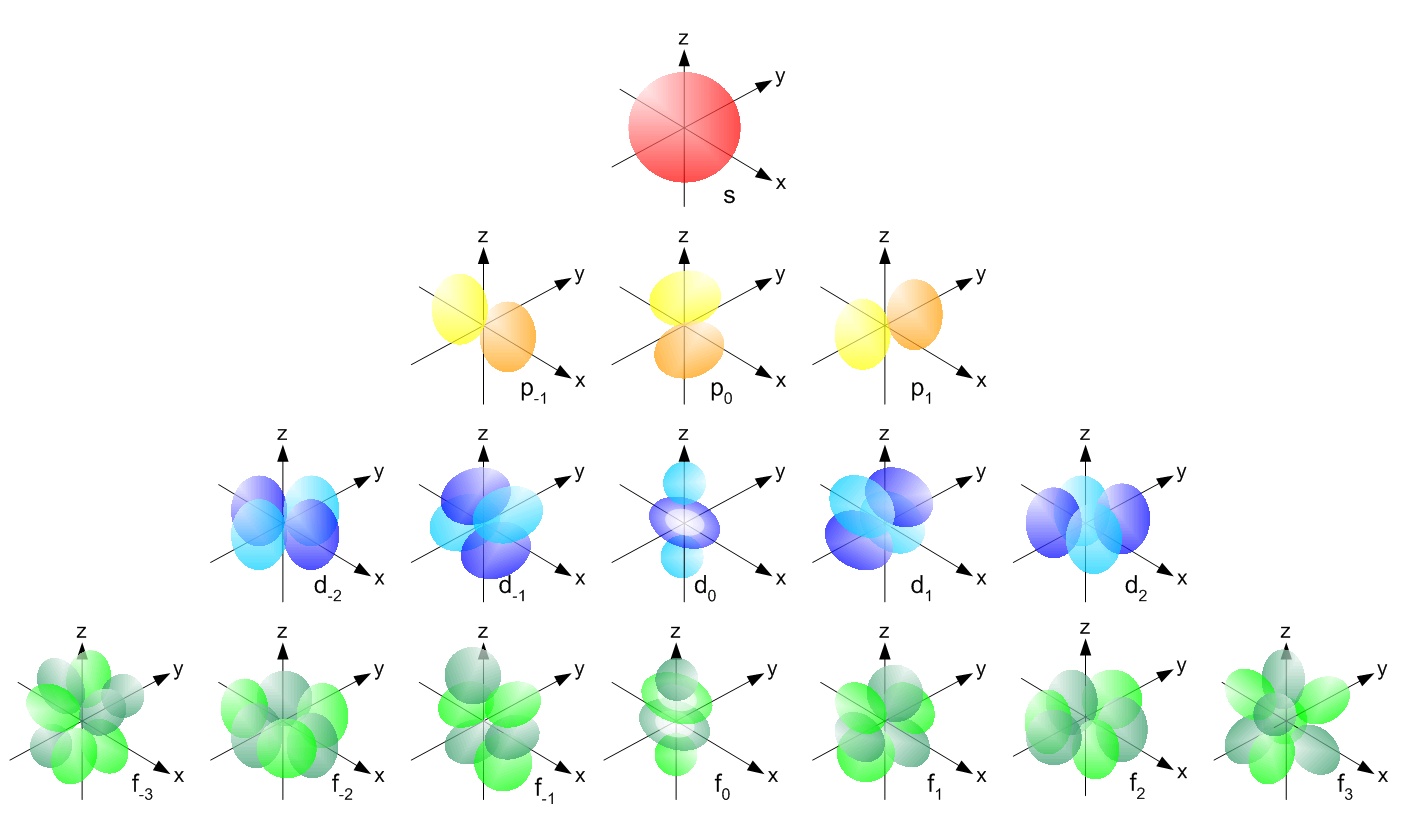
In the first post about atomic orbitals, it was mentioned that only atomic orbitals with the same symmetry can overlap to form molecular orbitals. For instance, s atomic orbitals form molecular orbitals with s atomic orbitals, p_x atomic orbitals with p_x atomic orbitals, and so on.

However, exceptions to this rule do exist.

MO diagram for nitrogen gas

Looking at the MO diagram above, Nitrogen gas obviously does not follow the rule because the 2s atomic orbitals are forming molecular orbitals with the 2p atomic orbitals. But how is this possible?? How come nitrogen gas can defy the basic rules of MO theory??

This is due to magical phenomena known as s-p mixing!

So, what is s-p mixing? This is a special process that only happen in elements where the s atomic orbital is very close in energy to the p atomic orbital. In this case, this usually happens to elements found before oxygen in the periodic table (hint: see nitrogen).

Diagram showing MO diagram before (a) and after (b) s-p mixing

The diagram above shows the MO diagram of a homonuclear diatomic compound before and after s-p mixing.

For S-P mixing to occur, the 2 interacting orbitals must be of the same symmetry and of similar energy. From the diagram above, we can see that the labelled orbitals are able to interact as they are of the same symmetry as labelled. Since they can interact, they must be of similar energy. A key point to note is that the greatest interaction occurs when the energy gap between the 2 interacting orbitals is the smallest.  Such an interaction occurs between 2σg and 3σg as they are closest in energy.

Comparing (a) and (b), it is evident that s-p mixing lowers the energy level of the 2σ orbitals, thereby stablising them. At the same time, the 3σ orbitals are raised in energy. This way, the 3σ bonding orbital is higher in energy than the 1π bonding orbital. Thus following the Aufbau principle, the 1π bonding orbitals are filled before the 3σ bonding orbital. Thus, s-p mixing can change the magnetism of a compound.

One example of a compound that changes magnetism after s-p mixing is B₂ as shown below:

MO diagram for B2 for no s-p mixing

MO diagram for B2 for s-p mixing

As seen, if s-p mixing occurs, B₂  will be paramagnetic. This is because the electrons fill the 2π bonding orbitals singly before pairing up. Whereas in the non s-p mixing state, there is only one σ bonding orbital created by the p atomic orbitals and that means that the electrons pair up to fill the σ bonding orbital up completely. Therefore, diamagnetism is observed.

S-p mixing might not be prevalent, however, it can be useful to explain why some elements do not follow the expected trend of magnetism.

Heteronuclear diatomic molecules are composed of two atoms of two different elements. The same electronic shell of the two atoms may not be of the same energy. That being said, it is not necessary for the electronic orbitals of the same shell to interact to give molecular orbitals. In fact, it is not necessary for the two 1s orbitals to interact. the 1s orbital may interact with other electronic orbitals, for example, this can be seen in the MO diagram of HF, below.

Figure 1: Molecular orbital of HF (Courtesy of chemwiki.ucdavis.edu)

The 1s orbital of H is of much similar energy to that of 2p in F. Therefore, interaction between the 1s and 2p orbitals takes place to form the molecular orbital of HF. Such electronic orbital interactions is common in heteronuclear diatomic as the electronic orbitals usually differ in energy levels.

In the molecular orbitals formed, a bonding and an anti-bonding molecular is formed. The molecules, H and F, contribute differently to each of these molecular orbitals. H contributes more to the anti-bonding orbitals as it is closer in energy to it. Likewise, F contributes moreto the bonding molecular orbital. The unequal contribution means that the covalent bond has a certain degree of ionic character.

Yes, so.. Do not be surprised the next time you see a 1s interacting with another 2p, 3s, 3p, who knows what orbital!

Apart from the magical process of s-p mixing, another magical process happens during the formation of molecular orbitals – sp-hybridisation!

To summarise, there are three main types of s-p hybrids available and they are as follows:

• sp³
• sp²
• sp

The shapes and angles of the hybrid atomic orbitals formed from s-p hybridisation are summarised below.

Bond angle and shapes associates with sp, sp2 and sp3 hybridisation

Sp³ hybridisation

One s orbital and three p orbitals hybridise to form four degenerate sp³ hybrid atomic orbitals (HAOs). The HAOs point towards the corners of a tetrahedron, thus, forming tetrahedral shape upon forming molecular orbitals. The bond angle in compounds with sp³ hybridisation is 109.5^o, allowing the compound to be more stable.

One example of a sp³ hybridised compound is C₂H₆.

Atomic orbitals overlap in C2H6

Sp² hybridisation

Sp² hybridised compounds are planar with a bond angle of 120^o. This is because three degenerate sp² hybrid atomic orbitals are produced.

One of the sp² hybridised compounds are CH₂O.

Atomic orbitals overlap in CH2O

Sp hybridisation

Sp hybridised compounds are also planar, with a bond angle of 180^o that will keep bond pairs as far away from each as possible.

An example of a sp hybridised compound is a C₂H₂.

Atomic orbitals overlap in C2H2